Chapter 1: Introduction to Projectile Motion

Projectile motion is a fascinating topic in physics that often arises in video analysis contexts. This scenario typically occurs when time data is unreliable, particularly if the motion appears to be in slow motion. Before diving into the specifics of the trajectory equation, let's discuss the standard approach for video analysis involving projectile motion.

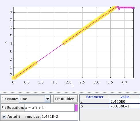
Initially, one would gather (x, y, t) data for each frame to create two separate plots. The first plot would illustrate horizontal position against time, which should yield a straight line. This linearity indicates zero acceleration, and the slope of the line represents horizontal velocity.

For example, consider the horizontal position of Red from Angry Birds in the following plot:

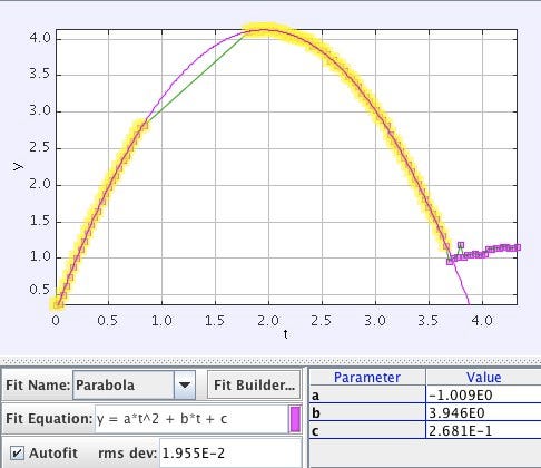
The next step is to plot vertical position against time, which should resemble a parabolic curve. Fitting a quadratic equation to this data allows for the determination of vertical acceleration, as demonstrated in another example from Angry Birds.

However, if the time data is poor, we may need to derive information from an x-vs-y plot, which represents the projectile's trajectory. For our analysis, let’s make some key assumptions:

1. We are dealing with a ball as our projectile.
2. The ball begins at an initial position of (x0, y0).
3. It is launched with a certain initial velocity (v0) at an angle (θ) above the horizontal.
4. The ground is defined as y = 0 m.
5. The vertical acceleration is -g (where g = 9.8 m/s²).
6. The motion starts at t = 0 seconds to simplify our equations.

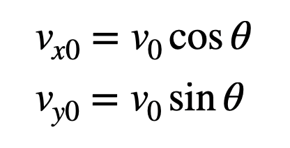
Now, let’s delve into the physics behind the motion. The initial velocity can be separated into its x- and y-components:

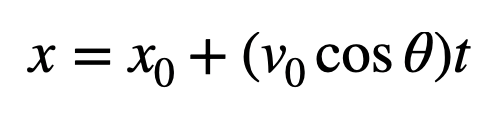
For the x-direction, we can apply the following kinematic equation:

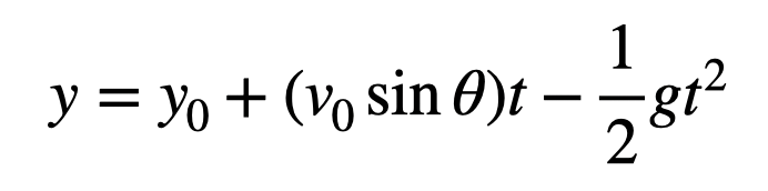
In the y-direction, we use:

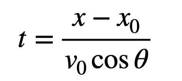
To derive the trajectory equation, we need to eliminate time (t) from these equations. We can start by rearranging the x-motion equation to solve for t.

Now, we can substitute this expression into the y-motion equation.

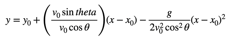
Notice how the velocity terms cancel out, resulting in a relation involving sine and cosine, which simplifies to tangent.

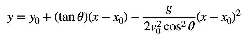
This formulation enables us to express the trajectory equation in a standard quadratic format, assuming the ball starts at x = 0.

Here, A, B, and C represent the fitting coefficients. The coefficient A can be derived as follows:

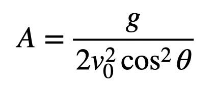
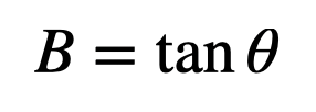
If we have the trajectory data plotted, we can ascertain the acceleration. This analysis presumes knowledge of both the launch velocity and the angle. Notably, the angle can be extracted from the B term:

Determining the launch velocity, however, is less straightforward. Knowing the vertical acceleration could facilitate this calculation, or potentially, the velocity might be obtained from other methods.

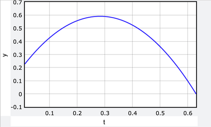
Let's put this theory to the test. While video data could be valuable, for simplicity, I will create a plot using Python. Below is a depiction of a ball launched from an initial position of x = 0 meters, producing the expected vertical position over time.

Next, I will plot two trajectory lines: one derived from traditional numerical calculations (x vs. y) and the other from the trajectory equation we previously solved. Here’s the resulting plot.

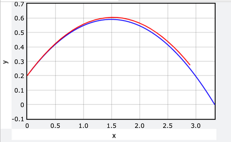
Although the plots may not perfectly align, adjustments can be made to ensure accuracy, demonstrating the validity of the derived equations.

Chapter 2: Video Analysis Techniques

To further illustrate the concepts discussed, check out the following video resources.

The first video titled "Trajectory of a projectile without drag" provides a visual understanding of projectile motion without external forces affecting it.

The second video, "Equation of Trajectory - Kinematics," delves into the mathematical foundations of projectile trajectories, enhancing your comprehension of the equations involved.

Originally published at http://rhettallain.com on March 29, 2020.