Understanding the Decision Tree Algorithm: A Comprehensive Guide
Written on
Chapter 1: Introduction to Decision Trees
The decision tree algorithm is a widely used technique in machine learning that can handle both linear and non-linear datasets effectively. It is applicable for tasks involving classification and regression. With an array of libraries available in Python and R, implementing decision trees has become accessible even for those unfamiliar with the underlying principles. However, grasping the fundamental workings of this algorithm is crucial for making informed choices about its application.
In this article, we will explore:
- A general overview of how decision trees operate: While this initial overview may seem abstract, a detailed example will follow to clarify the concepts.
- A practical example and the mathematical basis for decision-making within a decision tree: This section will illustrate how the decision tree algorithm arrives at conclusions through calculations.
Section 1.1: Mechanism of Decision Trees
The functioning of the decision tree algorithm revolves around making choices based on feature conditions. Each node represents a test on an attribute, branches indicate the outcomes of these tests, and leaf nodes signify the final decisions derived from the conditions.
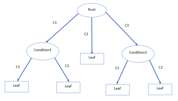
As depicted in the diagram, the process begins with a root condition, leading to multiple branches (C1, C2, C3). The number of branches can vary depending on the root node's feature classes. The branches culminate in leaf nodes, which represent the ultimate decisions or predictions. For instance, C1 and C3 lead to Condition1 and Condition2, which represent distinct features. The data will be further divided based on the categories in Condition1 and Condition3, as shown in the illustration above.
Before diving deeper, let's clarify some essential terms:
- Root Nodes: The starting point of the decision tree, where the first feature initiates the data splitting.
- Decision Nodes: These nodes, such as ‘Condition1’ and ‘Condition3’, are formed after splitting from the root node, allowing for further data division.
- Leaf Nodes: The final nodes where decisions are made, with no additional splitting possible. In the illustration, Decision2 and Decision3 are classified as leaf nodes.
Section 1.2: Practical Example and Calculations
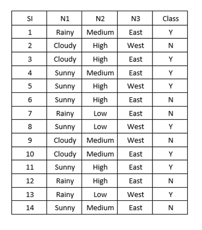
To demonstrate the decision-making process, we will use a synthetic dataset featuring a binary class and three categorical variables: N1, N2, and N3.
With this dataset in hand, the initial step is to select a root node. The question arises: How do we determine which feature should serve as the root? Should we simply choose N1 because it appears first in the dataset?
Not quite. To make an informed choice regarding the root node, we must delve into the concept of information gain. This statistical measure helps us assess which feature will best reduce uncertainty when classifying data.
The selection of test attributes relies on several purity measures, including:
- Information Gain
- Gain Ratio
- Gini Index
In this discussion, we will focus on Information Gain.
Imagine a scenario where 10 friends are trying to decide between watching a movie or going out. If five wish to watch a movie and the other five prefer to go out, reaching a consensus is challenging. However, if a large majority (8 or 9) want to watch a movie, making a decision becomes straightforward. In decision trees, a dataset is considered pure when all classes belong to either "yes" or "no". Conversely, if they are evenly split (50% each), the dataset is deemed impure, resulting in uncertainty in decision-making.
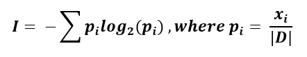
Information gain quantifies the reduction of uncertainty associated with a feature, aiding in the identification of a suitable root node. This calculation is based on a measure called entropy.
The formula for entropy is as follows:
Let’s go through a detailed example using our synthetic dataset to identify the root node.
We have a total of 14 data entries, consisting of 8 "yes" classes and 6 "no" classes.
Calculating the overall entropy yields:
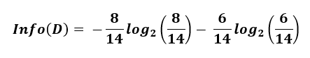
The resulting entropy is 0.985, representing the parent entropy.
Next, we will compute the entropy for each of the three variables (N1, N2, N3) individually to determine which feature should be the root node.
Starting with N1, we analyze the breakdown:
- Rainy: 4 entries (2 "Y"s and 2 "N"s)
- Sunny: 4 entries (2 "Y"s and 2 "N"s)
- Cloudy: 6 entries (4 "Y"s and 2 "N"s)
The information required to classify the dataset based on N1 is calculated as follows:
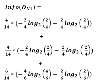
This results in an information gain of:
Info_gain(N1) = 0.985 - 0.964 = 0.021
Subsequently, we can calculate the information gains for N2 and N3, resulting in values of 0.012 and 0.001, respectively.
From this analysis, N1 emerges as the feature with the highest information gain, positioning it as the root node.
At this juncture, our decision tree appears as follows:
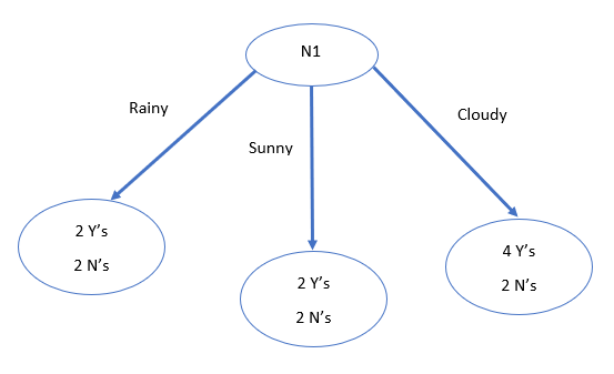
Now that we have established the root node, we can further split the data based on the conditions. Observing the entropy values, we note that the "Rainy" and "Sunny" conditions exhibit high entropy due to the equal distribution of "Y"s and "N"s. In contrast, the "Cloudy" condition suggests a lower entropy, indicating a likelihood of a "Y" class.
The next step involves calculating the information gain for the subnodes to determine subsequent splits.
Section 1.3: Stopping Criteria for Splitting
While we have explored the splitting process for features, the example dataset contains only three features. In real-world applications, datasets may encompass a far greater number of features, which can lead to complex trees prone to overfitting and longer computation times.
To mitigate this, the max_depth parameter in the scikit-learn library allows for tree depth control. A larger max_depth results in a more extensive tree, while limiting the depth can prevent overfitting. Additionally, the max_features parameter enables the selection of a maximum number of features utilized in the tree construction.
Refer to the library documentation for additional parameters and customization options.
Chapter 2: Advantages and Disadvantages of Decision Trees
The video "Decision Tree Classification Clearly Explained!" provides a clear visual overview of the decision tree algorithm's workings. It serves as a valuable resource for understanding the concept.
Major Advantages of Decision Trees:
- Clear visualization of predictions, making it easy to convey insights to stakeholders.
- No need for feature scaling.
- Non-linear relationships between dependent and independent variables do not hinder performance.
- Automatic handling of outliers and missing values.
Major Disadvantages of Decision Trees:
- Prone to overfitting, leading to high variance and prediction errors.
- Sensitivity to noise; small changes in data can significantly alter the tree structure.
- Not well-suited for large datasets, which may complicate the algorithm and increase the risk of overfitting.
The second video, "How Do Decision Trees Work (Simple Explanation)," offers a simplified overview of the learning and training process behind decision trees.
Conclusion
Both Python and R provide excellent libraries for implementing popular machine learning algorithms, making it accessible for practitioners. However, understanding the underlying mechanisms greatly enhances decision-making regarding the selection of appropriate algorithms for specific projects.
More Reading
- Multiclass Classification Algorithm from Scratch with a Project in Python: Step by Step Guide
- Details of Violinplot and Relplot in Seaborn
- A Complete K Mean Clustering Algorithm From Scratch in Python: Step by Step Guide
- Stochastic Gradient Descent: Explanation and Complete Implementation from Scratch
- A Complete Anomaly Detection Algorithm From Scratch in Python: Step by Step Guide
- Dissecting 1-Way ANOVA and ANCOVA with Examples in R
- A Complete Sentiment Analysis Algorithm in Python with Amazon Product Review Data: Step by Step