What is Transfer Learning?

In practice, very few practitioners build a deep neural network from scratch due to the difficulty of obtaining a large dataset with enough samples for each category. Instead, many opt to pre-train a DNN on extensive datasets such as ImageNet, which contains 1.2 million images across 1,000 classes. These pre-trained models can then be adapted for specific tasks like image classification on smaller datasets. This technique is known as transfer learning and has become a fundamental tool in machine learning, gaining traction as a method to enhance the performance of DNNs trained on limited data.

Now, let’s dive into the implementation of a DNN utilizing transfer learning on a small dataset. I will utilize the PyTorch framework to train the model on the publicly available Flower dataset, which comprises 4,317 images categorized into five distinct classes.

Implementing a DNN with a Small Dataset

For this tutorial, I will use Google Colab, which allows users to write and execute Python code through a web browser by hosting a Jupyter notebook. If you're using Colab, make sure to switch the runtime to utilize a GPU for better performance.

Can AI Writers Replace Human Writers?

Human Writer vs AI Writer

Steps to Train a DNN for a Small Dataset

Step 1: Download and Extract the Datasets

The Flower dataset contains five categories: daisy, dandelion, roses, sunflowers, and tulips. This dataset, built by Alexander Mamaev, is available for research purposes. Our goal is to construct a DNN that classifies these flower images into their respective categories.

# Download the dataset

# Unzip the dataset

!unzip /content/flower-photos.zip

Step 2: Import Necessary Libraries

We will leverage PyTorch libraries such as torch, torch.nn, and torch.nn.functional. We’ll also utilize numpy and torchvision for dataset pre-processing and model handling. For visualizations, we'll use matplotlib.pyplot.

import torch

import matplotlib.pyplot as plt

import numpy as np

import torch.nn.functional as F

from torch import nn

from torchvision import datasets, transforms, models

Step 3: Set Hyperparameters

Here, we will define the hyperparameters, including the number of epochs, batch size, and learning rate.

# Hyperparameters

epochs = 10

batch_size = 32

learning_rate = 0.0001

Step 4: Determine the Device

This command checks if CUDA is available. If so, it will remain True for the entire program.

# For GPU

device = torch.device("cuda:0" if torch.cuda.is_available() else "cpu")

Step 5: Prepare the Dataset

Once the dataset is downloaded, we must preprocess it before feeding it into the neural network. The torch.utils.data.DataLoader class is integral to PyTorch’s data loading capabilities, providing a Python iterable over the dataset. We need to normalize the data to maintain it within a suitable range, which enhances the model's learning efficiency.

# Prepare the dataset

transform_train = transforms.Compose([

transforms.Resize((224, 224)),

transforms.RandomHorizontalFlip(),

transforms.RandomAffine(0, shear=10, scale=(0.8, 1.2)),

transforms.ColorJitter(brightness=1, contrast=1, saturation=1),

transforms.ToTensor(),

transforms.Normalize((0.5, 0.5, 0.5), (0.5, 0.5, 0.5))

])

transform = transforms.Compose([

transforms.Resize((224, 224)),

transforms.ToTensor(),

transforms.Normalize((0.5, 0.5, 0.5), (0.5, 0.5, 0.5))

])

train_dataset = datasets.ImageFolder('/content/flower_photos/train', transform=transform_train)

val_dataset = datasets.ImageFolder('/content/flower_photos/test', transform=transform)

train_loader = torch.utils.data.DataLoader(train_dataset, batch_size=batch_size, shuffle=True)

val_loader = torch.utils.data.DataLoader(val_dataset, batch_size=batch_size, shuffle=False)

print(len(train_dataset))

print(len(val_dataset))

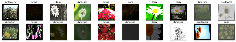
Step 6: Visualize the Dataset Samples

To visualize some samples from our dataset, we will define a helper function.

# Helper function to visualize the data

def im_convert(tensor):

image = tensor.cpu().clone().detach().numpy()

image = image.transpose(1, 2, 0)

image = image * np.array((0.5, 0.5, 0.5)) + np.array((0.5, 0.5, 0.5))

image = image.clip(0, 1)

return image

The Flower dataset comprises five classes: daisy, dandelion, roses, sunflowers, and tulips. Let's visualize a few images from our training set.

# Visualize training images

classes = ('daisy', 'dandelion', 'roses', 'sunflowers', 'tulips')

dataiter = iter(train_loader)

images, labels = dataiter.next()

fig = plt.figure(figsize=(25, 4))

for idx in np.arange(20):

ax = fig.add_subplot(2, 10, idx + 1, xticks=[], yticks=[])

plt.imshow(im_convert(images[idx]))

ax.set_title(classes[labels[idx].item()])

Step 7: Instantiate the Model

We will utilize the pre-trained AlexNet architecture for our dataset.

model = models.alexnet(pretrained=True)

print(model)

Step 8: Modify the Model for Our Dataset

Given that AlexNet was trained on ImageNet with 1,000 classes, we will adjust the final fully connected layer for our five classes.

n_inputs = model.classifier[6].in_features

last_layer = nn.Linear(n_inputs, len(classes))

model.classifier[6] = last_layer

model.to(device)

Step 9: Define Loss Function and Optimizer

We will implement the cross-entropy loss and the Adam optimizer for our model.

criterion = nn.CrossEntropyLoss()

optimizer = torch.optim.Adam(model.parameters(), lr=learning_rate)

Step 10: Train the Network

To train the network, we will perform a forward pass, compute the loss, calculate gradients, and update the weights accordingly.

# Track loss and accuracy

running_loss_history = []

running_corrects_history = []

val_running_loss_history = []

val_running_corrects_history = []

class_total = list(0. for i in range(5))

for e in range(epochs):

running_loss = 0.0

running_corrects = 0.0

val_running_loss = 0.0

val_running_corrects = 0.0

# Train the model

for inputs, labels in train_loader:

inputs = inputs.to(device)

labels = labels.to(device)

outputs = model(inputs)

loss = criterion(outputs, labels)

optimizer.zero_grad()

loss.backward()

optimizer.step()

_, preds = torch.max(outputs, 1)

running_loss += loss.item()

running_corrects += torch.sum(preds == labels.data)

# Validation phase

with torch.no_grad():

for val_inputs, val_labels in val_loader:

val_inputs = val_inputs.to(device)

val_labels = val_labels.to(device)

val_outputs = model(val_inputs)

val_loss = criterion(val_outputs, val_labels)

_, val_preds = torch.max(val_outputs, 1)

val_running_loss += val_loss.item()

val_running_corrects += torch.sum(val_preds == val_labels.data)

epoch_loss = running_loss / len(train_loader.dataset)

epoch_acc = running_corrects.float() / len(train_loader.dataset)

running_loss_history.append(epoch_loss)

running_corrects_history.append(epoch_acc)

val_epoch_loss = val_running_loss / len(val_loader.dataset)

val_epoch_acc = val_running_corrects.float() / len(val_loader.dataset)

val_running_loss_history.append(val_epoch_loss)

val_running_corrects_history.append(val_epoch_acc)

print('Epoch:', (e + 1))

print('Training Loss: {:.4f}, Accuracy: {:.4f}'.format(epoch_loss, epoch_acc.item()))

print('Validation Loss: {:.4f}, Validation Accuracy: {:.4f}'.format(val_epoch_loss, val_epoch_acc.item()))

Step 11: Evaluate Model Performance

Now we will assess the accuracy of our model on the test images.

total_images = 0

confusion_matrix = np.zeros([5, 5], int)

with torch.no_grad():

for data in val_loader:

images, labels = data

images = images.to(device)

labels = labels.to(device)

outputs = model(images)

_, predicted = torch.max(outputs.data, 1)

total_images += labels.size(0)

total_correct += (predicted == labels).sum().item()

for i, l in enumerate(labels):

confusion_matrix[l.item(), predicted[i].item()] += 1

model_accuracy = total_correct / total_images * 100

print('Model Accuracy on {} test images: {:.2f}%'.format(total_images, model_accuracy))

We achieved a classification accuracy of 81.48% on our flower dataset.

Step 12: Class-Wise Accuracy and Confusion Matrix

To obtain class-wise accuracy, the following code can be utilized.

print('{0:5s} : {1}'.format('Category', 'Accuracy'))

for i, r in enumerate(confusion_matrix):

print('{0:5s} : {1:.1f}'.format(classes[i], r[i] / np.sum(r) * 100))

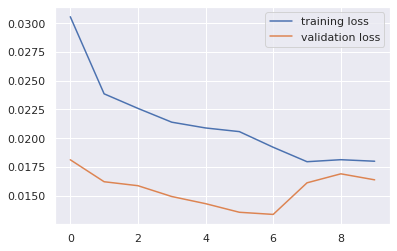
Step 13: Plot Training and Validation Metrics

Lastly, we can plot the training and validation loss and accuracy curves.

import seaborn as sns

sns.set()

plt.plot(running_loss_history, label='Training Loss')

plt.plot(val_running_loss_history, label='Validation Loss')

plt.legend()

plt.plot(running_corrects_history, label='Training Accuracy')

plt.plot(val_running_corrects_history, label='Validation Accuracy')

plt.legend()

Step 14 (Optional): Classify an Image from the Web

You can also classify an image from the web using the trained model.

import PIL.ImageOps

import requests

from PIL import Image

response = requests.get(url, stream=True)

img = Image.open(response.raw)

plt.imshow(img)

img = transform(img)

plt.imshow(im_convert(img))

image = img.to(device).unsqueeze(0)

output = model(image)

_, pred = torch.max(output, 1)

print(classes[pred.item()])

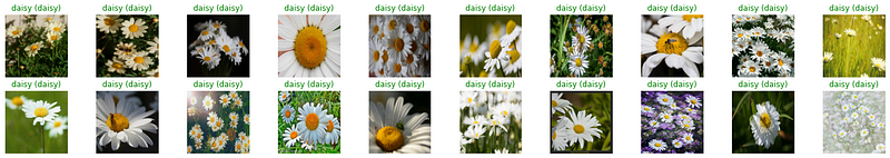
Step 15 (Optional): Visualize Classification Results

The following code can be used to visualize the test results alongside the ground truth classes and predicted classes.

dataiter = iter(val_loader)

images, labels = dataiter.next()

images = images.to(device)

labels = labels.to(device)

output = model(images)

_, preds = torch.max(output, 1)

fig = plt.figure(figsize=(25, 4))

for idx in np.arange(20):

ax = fig.add_subplot(2, 10, idx + 1, xticks=[], yticks=[])

plt.imshow(im_convert(images[idx]))

ax.set_title("{} ({})".format(str(classes[preds[idx].item()]), str(classes[labels[idx].item()])), color=("green" if preds[idx] == labels[idx] else "red"))

In this article, we've demonstrated how to implement a deep neural network on a small dataset. With only 4,317 images, we achieved approximately 81% classification accuracy in under one hour, provided you have access to a robust GPU.

Before You Go:

If you enjoy reading stories on Medium, consider supporting writers by becoming a member using my referral link. It's only $5 a month for unlimited access to all stories. If you sign up through this link, I’ll receive a small commission at no extra cost to you. Alternatively, you can support me through my tip jar on Ko-fi or PayPal.